Data Science Case Study: Music Popularity using Spotify API

This article has code from my GitHub notebook, you can find it here.

We all have our favorite artists, genres, and albums. Almost everyone, throughout the journey of life, hears a chord that strikes and perfectly resonates with them, despite the ever-changing nature of this "Journey". A lot of the time, we hear that rhythm with the stories a few particular artists are telling, and before you know it you have a new favorite artist.

Over the years, I have tried to maintain a habit of listening to new music now and then, and throughout the process, I have stumbled across very simple yet obvious realizations- perhaps, I did not understand the depth it carries before. There are multiple artists out there who work in the same way your artist does within a style of their own, and an overwhelmingly large amount of times these artists are still waiting for their "Big Break".

This case study aims to analyze statistically what makes a song popular and aims to quantify creativity into a measurable metric, which then can be utilized to highlight the talent that mathematically has the numbers to succeed. This case study embodies my value of using data to bring about a positive impact taking a small step towards fostering a supportive community.

Spotify - with its commitment to unlocking the creative potential of creators has a great deal of features that foster and support emerging talent. Features of smart shuffle, creating emerging talent playlists, and creating daily mixes for its members, showcase Spotify's commitment and steps towards nurturing and nourishing a community. This case study if coupled with a large database, could help serve this goal.

Throughout this article, I guide on the key aspects of my guided notebook and the intuition behind the steps. The data for this case study was taken from Statso; which is an organization by Aman Kharwal, focused on data science consulting. Shoutout to Aman for his incredible work, and continuous dedication to data science.

Let's get started.

Contents:

1. Data and Feature Analysis

2. Handling Multicollinearity

3. Model Training, Evaluation, and Selection

4. How can such a system be useful?

Part 1: Data and Feature Analysis

Let us first take a look at the features, we have-

spotify.columns

Index(['Unnamed: 0', 'Track Name', 'Artists', 'Album Name', 'Album ID',
       'Track ID', 'Popularity', 'Release Date', 'Duration (ms)', 'Explicit',
       'External URLs', 'Danceability', 'Energy', 'Key', 'Loudness', 'Mode',
       'Speechiness', 'Acousticness', 'Instrumentalness', 'Liveness',
       'Valence', 'Tempo'],
      dtype='object')

The unnamed column is just an index we can directly remove it, and for the column Release Date - we can convert it into a continuous integer range.

# removing the unnamed column
spotify_data = spotify.drop(columns='Unnamed: 0')
# Using the release data, for which need to convert it into datetime format
spotify_data['Release Date'] = pd.to_datetime(spotify_data['Release Date'])
spotify_data['Release Date ordinal'] = spotify_data['Release Date'].apply(lambda x: x.toordinal())

Now let us analyze how each of these features varies with popularity,

features = ['Duration (ms)','Danceability','Energy','Loudness','Speechiness','Acousticness','Instrumentalness','Liveness','Tempo','Valence', 'Release Date ordinal']
for feature in features:
    plt.figure(figsize=(8,5))
    sns.regplot(data = spotify_data, x=feature, y='Popularity', scatter_kws={'s': 50}, line_kws={'color': 'red'})
    plt.title(f'Popularity vs {feature}')
    plt.show()

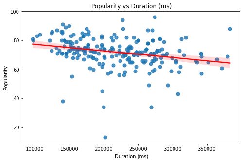
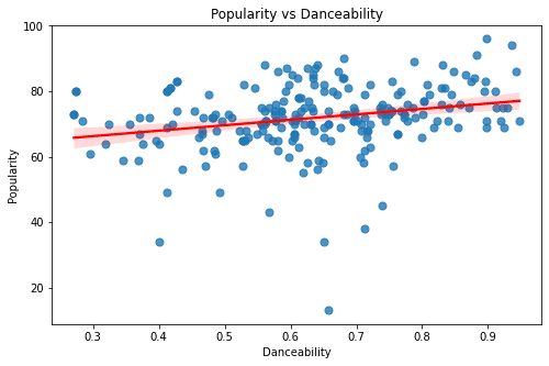
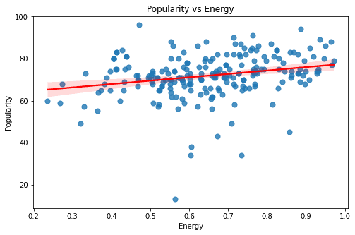
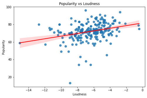
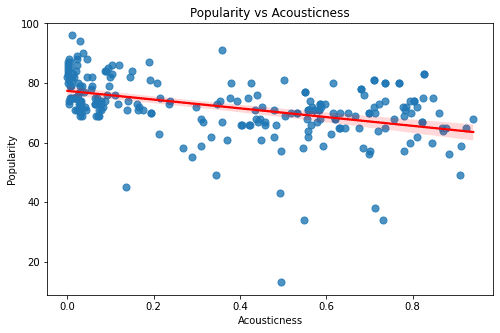
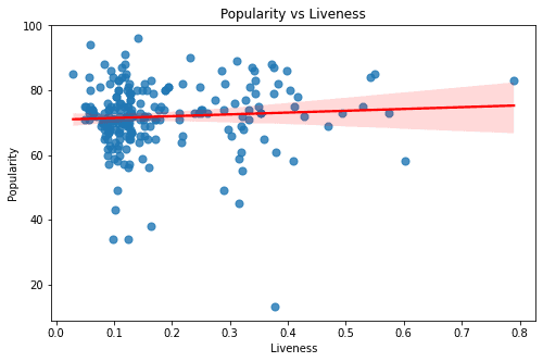
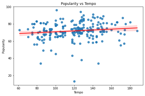
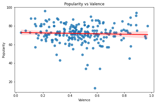
The above graphs are of the features - Duration, Valence, Tempo, Liveness, Acousticness, Loudness, Energy, and Danceability. All of these graphs seem to have a rather sporadic pattern and a small magnitude of correlation. Looking at these graphs one thing is for sure - Linear Models can only explain a part of our target variable - popularity.

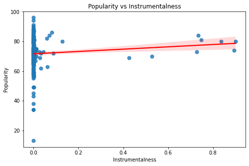
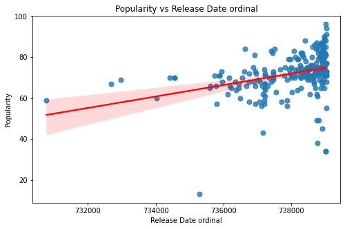
For the remaining two features: Instrumentalness & Release Date the data is rather cluttered to one side, which is a potential bias in the data.

Looking at the features, naturally, it is safe to assume there might be a lot of overlap among these features - meaning there might be a correlation between the features themselves. This can cause problems in our machine learning such as overfitting - prioritizing the patterns that are being repeated.

So let us check, the correlation between the features.

# Finding the correlation
numeric_columns = spotify_data.select_dtypes(include=['float64', 'int64']).columns
numeric_data = spotify_data[numeric_columns]

corr_matrix = numeric_data.corr()

plt.figure(figsize=(12, 8))
sns.heatmap(corr_matrix, annot=True, cmap='coolwarm', fmt='.2f', linewidths=0.5)
plt.title('Correlation Matrix')
plt.show()

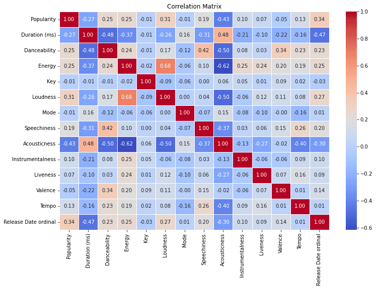
I can see there are some high correlation magnitudes. The highest one is Loudness and Energy - which only makes sense. The other one is the relationship between acousticness and energy. From these two I am keeping the relation between acousticness and energy as I think they both capture different variances. However, for loudness and energy, it is safe to assume that these two have much more overlap.

Part 2: Handling Multicollinearity

Principal Component Analysis is a method of feature engineering that analyzes principal components from multiple features, reducing the dimensions.

To solve the problem of multicolinearity, let us perform PCA to create a new feature 'energy_loudness_pca' which captures the principal component from both the features 'Energy' & 'Loudness'.

pca = PCA(n_components=1)
spotify_data['energy_loudness_pca'] = pca.fit_transform(spotify_data[['Energy', 'Loudness']])

Looking at the correlation plot again:

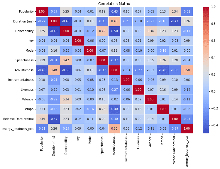
After performing PCA, the multicollinearity problem between energy and loudness is resolved as well as the correlation of Acousticness with energy_loudness_pca is also reduced. This solves the problem of multicollinearity.

Now, to determine which features to keep in our machine learning model. As previously discussed, the goal of this model is to determine what makes a song popular and hopefully use specific song characteristics to determine if the song would be popular or not. To select the features, let us compare the correlation of these features with the r-squared coefficient. The r-squared coefficient helps explain, how much % of the variance is in variable 1-(Popularity) and variable 2 (the other variable)

#Now using these columns with correlation coefficient and computing their r-square to determine the features to use:
import numpy as np
linear_regression_results = pd.DataFrame(columns=['Feature','Correlation','r-squared'])
new_features = ['Duration (ms)', 'Danceability', 'Key', 'Mode',
       'Speechiness', 'Acousticness', 'Instrumentalness', 'Liveness',
       'Valence', 'Tempo', 'Release Date ordinal', 'energy_loudness_pca']



for feature in new_features:
    correlation = numeric_data['Popularity'].corr(numeric_data[feature])



    slope, intercept = np.polyfit(numeric_data[feature],numeric_data['Popularity'],1)

    predicted_values = slope * numeric_data[feature] + intercept

    residuals = numeric_data['Popularity'] - predicted_values
    ss_total = np.sum((numeric_data['Popularity'] - np.mean(numeric_data[feature]))**2)
    ss_residual = np.sum(residuals**2)

    r_squared_2 = 1 - (ss_residual/ss_total)

    new_rows_2 = pd.DataFrame({'Feature':[feature],'Correlation': [correlation],'r-squared':[r_squared_2]})
    linear_regression_results = pd.concat([linear_regression_results,new_rows_2],ignore_index=True)

# Sorting by absolute mangitude
linear_regression_results['Abs_Correlation'] = linear_regression_results['Correlation'].abs()
sorted_results = linear_regression_results.sort_values(by=['Abs_Correlation', 'r-squared'], ascending=[False, False]).reset_index(drop=True)
sorted_results = sorted_results.drop(columns=['Abs_Correlation'])

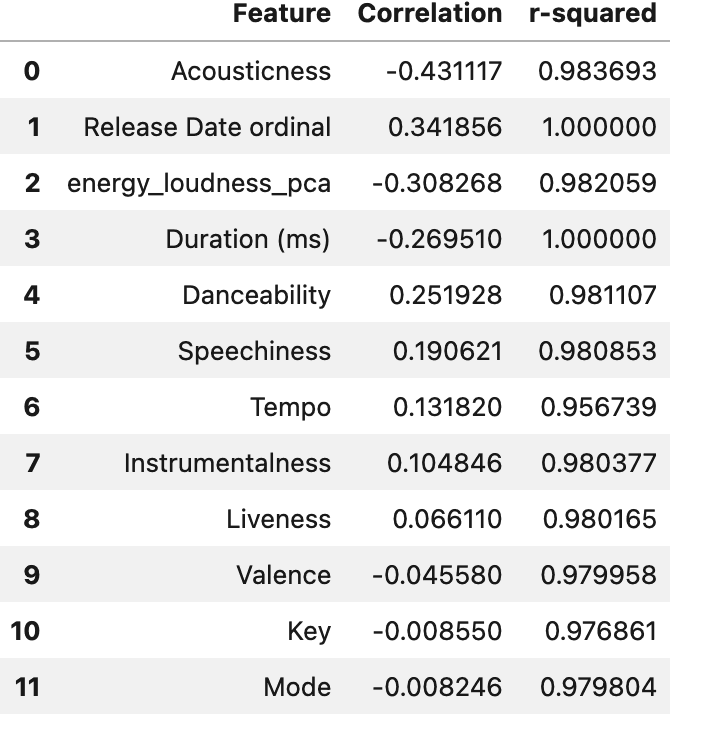
We can drop the columns Key, and Mode as they have super low correlation.

Part 3: Model Training, Evaluation and Selection

• Three models that I selected

• Performance analysis

• Why did they perform the way they performed

To train and evaluate I chose three models- Linear Regression as a baseline, and then two tree-based models Random Forest Classifier and XGBoost. Using intuition, I think tree-based models make the most sense here as trees work well within a diverse set of features. Linear regression is not expected to perform well in this scenario as from the earlier graphs it clearly did not explain all of the variations of the data.

After training the model, and evaluating the scores, Random Forest and XGBoost performed better than linear regression, those two models were very close in their scores. I then performed a grid search to find the best parameters for both of the models and here were the complete results.

                  Model      RMSE  R-squared
0     Linear Regression  7.972830   0.044975
1         Random Forest  6.290022   0.405579
2               XGBoost  6.745217   0.316432
3  Random Forest (Best)  6.013741   0.456651
4        XGBoost (Best)  6.093559   0.442132

I further analyzed the Random Forest and XGBoost models with Error and Residual graphs.

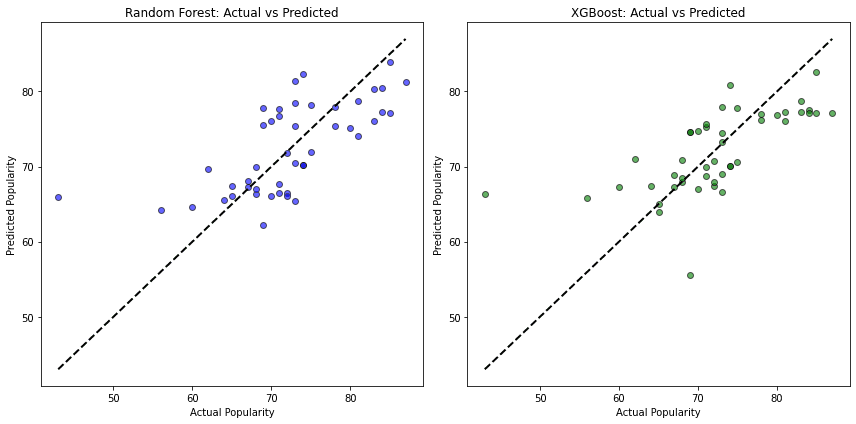
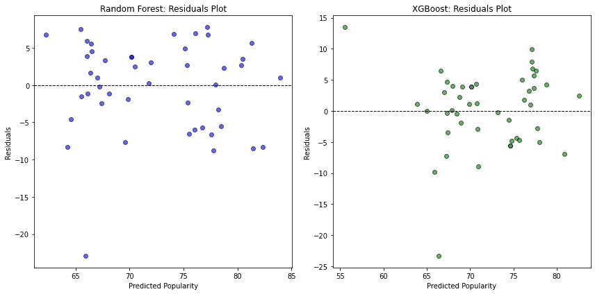
Analyzing the graphs both of these models have similar performance, however, these models are heavily impacted by the bias in the data that we discussed earlier, and the presence of outliers. The performance of this model can be significantly improved using more data, and more importantly unbiased data.

I went ahead and chose a random forest classifier for the demo of this app. You can input the name of the song, and the artist and it classifies the song into Not Popular, Moderately Popular, or Highly popular based on the numbers behind the songs. Test out the demo for yourself here!

Part 4: How can such a system be useful?

For music labels, this model offers a strategic advantage, enabling them to allocate resources to songs that are most likely to resonate with current audiences. By predicting which tracks align with listener trends, labels can optimize marketing budgets, schedule releases more effectively, and amplify songs with strong hit potential.

Independent artists can benefit greatly from such a tool as well, allowing them to make informed choices about their singles and anticipate how new releases might perform. For those without the backing of a major label, these insights can focus promotional efforts where they’ll be most impactful, maximizing reach and audience engagement.

Integrated into streaming platforms’ recommendation engines, this model could prioritize songs predicted to resonate, tailoring playlists to keep users engaged and boosting the discovery of emerging artists. Radio stations, too, could use predictions to curate playlists that balance familiar hits with fresh tracks, providing a dynamic listening experience that keeps audiences tuned in.

In essence, a popularity prediction model can act as a bridge between data and creativity, allowing music industry professionals to connect with audiences more effectively and shape their strategies in a rapidly evolving landscape.

Feel free to check out my Linkedin, and contact me for any queries. Thank you for reading through.